1. A Gentle Introduction to Summarizing Data
In this tutorial we are going to define some common terms and concepts including the basic types, or categories, of data. Then we'll learn how to describe a dataset. By the end you will be prepared to take the concepts here and use them to summarize the polling station list in the next module.
Data Terms
We begin by learning some common terms used in examining data.
Observation
A dataset contains information about "individuals". Each "individual" is called an "observation" or "case". In most datasets, each row contains information about an individual.
Variable
Any characteristic of an individual (i.e., observation) is called a variable. Some variables, like gender and job title, simply place individuals into categories. Others, like height or number of registered voters, take on numerical values for which we can do arithmetic. Next we'll take a closer look at the different types of data.
Data Types
Data is stored as different types, which are sometimes referred to as the "level of measurement". We need to understand the type of data because it helps us figure out how to properly summarize it. There are three types of data:
- Categorical or Nominal: These are data that have several categories and are not numerical (e.g., gender, ethnicity, constituency). For example, an election observation form might ask "Were you permitted to observe all day?" where the answer option is either "Yes" or "No". An election management body (EMB) might release a list of officials who are assigned to each polling station, and that list might contain the name and position of the official. The "position'" variable is likely to be categorical data (e.g., President, Deputy President, and Secretary).
- Ordinal: These are data with categories that go in a specific order or rank. For example, on many election observation forms, there is a questions that asks "How many people were assisted to vote?" where the answer options are "None", "Few", "Some", or "Many". "Many" is more than "Some", which is more than "None".
- Continuous or Interval: This kind of data has a continuous range of numbers. All data values are possible. For example, an election day observation form may ask for the number of registered voters for each polling station or the number of votes received for each candidate.
By first understanding what type of data a variable is, we can then decide how to best summarize or describe that variable.
Describing & Summarizing Data
Why do we summarize? We summarize data to "simplify" the data and quickly identify what looks "normal" and what looks odd. The distribution of a variable shows what values the variable takes and how often the variable takes these values.
The two most useful ways of describing the distribution of data are:
- The typical: This describes the center--or middle--of the data. This way of describing the center is also called a "measure of central tendency".
- The spread of the values around the center: This describes how densely the data is distributed around the center. This is also called a "measure of dispersion".
These two ways of describing the data are also referred to as descriptive statistics.
1. The Center: What is Typical? (Central Tendencies)
The three common ways of looking at the center are average (also called mean), mode and median. All three summarize a distribution of the data by describing the typical value of a variable (average), the most frequently repeated number (mode), or the number in the middle of all the other numbers in a data set (median).[1] In this module, we are going to focus on the average. The average is the most appropriate way to measure the center for interval/continuous data (e.g, numbers of registered voters). To calculate the average, we add up all the numbers for a variable and then divide by how many numbers there are. Put another way the average (mean) is the sum divided by the count.
Simple Example
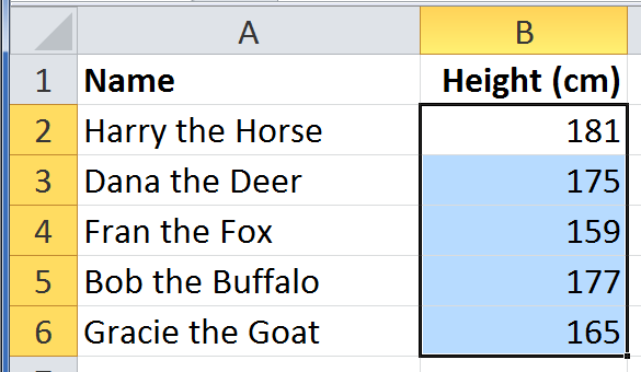
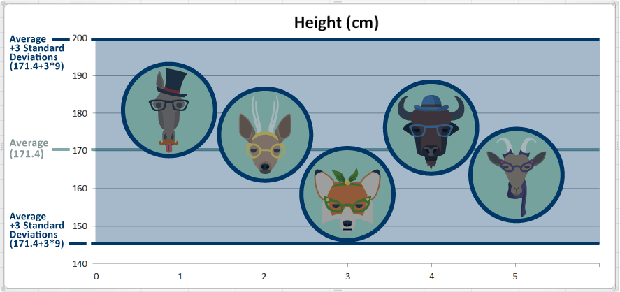
In the example dataset below, we have information about the names of some animals. We also have measurements of the height of each animal. The dataset has two variables -- name and height -- and five observations. Here is the dataset:
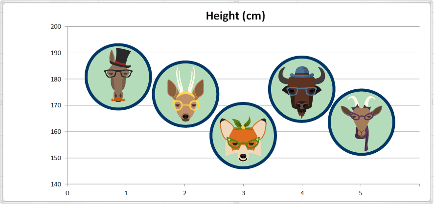
Here we've made a quick chart that plots the height of each animal:
To calculate the Average height (in cm) we sum up all the values and divide by the total count of observations:
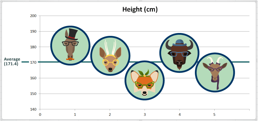
Average height = (181 + 175 + 159 + 177 + 165) ÷ 5 = 857 ÷ 5 = 171.4
The average value for height is 171.4 centimeters. Here we have added a reference line marking the average on our chart so we can see how that looks:
2. The Spread: How is the data distributed around the center? (Measures of Dispersion)
Looking at the spread of the distribution of data tells us about the amount of variation, or diversity, within the data. The three measures of the spread of the data are the range, the standard deviation, and the variance.
Range
This is the difference between the largest and the smallest values. It is the distance between the extremes. To calculate the range, we take the maximum value and subtract the minimum value.
In our height dataset, what is the largest value (maximum)? 181 cm
In the same example, what is the smallest value (minimum)? 159 cm
The range in our small dataset of heights is 181 - 159 = 22 cm
Here we added some reference lines on the chart to indicate the maximum and minimum:
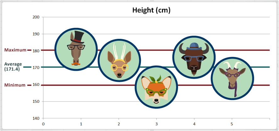
In practical terms, the animal with the maximum value is the tallest, and the animal with the minimum value is the shortest. So Harry the Horse is the tallest, and Fran the Fox is the shortest.

While the range gives us the endpoints (i.e., extremes), it does not tell us anything about how tightly or loosely the data are distributed between those two endpoints. We also do not know whether more of the data is closer to the average, the maximum or the minimum. From our chart, it looks like just over half of the animals are tall (i.e., above the average height).
Two other related measures of dispersion--the variance and the standard deviation--can help us answer these questions. They provide a numerical summary of how much the data are scattered.
Standard Deviation
The standard deviation provides us with a standard way of knowing what is normal[2] given the average. A really helpful attribute of the standard deviation is that it is expressed in the same units as the data itself. The standard deviation is like an "index of variability," because it is proportional to the scatter of the data. The standard deviation is larger for more diverse distributions (i.e., the data are widely scattered). The standard deviation is smaller for less diverse distributions (i.e., the data are clustered together).
The standard deviation is very useful for understanding the spread of a variable. For most "normally" distributed data, generally almost all of the values will be within three standard deviations of the average. In statistics, this is sometimes referred to as the 68-95-99.7 rule. About 68.27% of the values lie within 1 standard deviation of the average (mean). Similarly, approximately 95.45% of the values lie within 2 standard deviations of the mean. Nearly all (99.73%) of the values lie within 3 standard deviations of the mean.
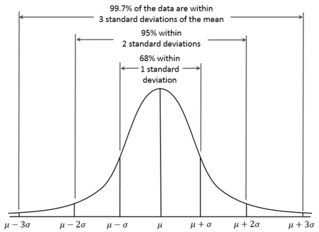
A diagram of the 68-95-99.7 rule from wikipedia
In Module 3, we use Excel to summarize the data in the 2008 polling station list.
In the sample animal heights dataset, we've calculated the standard deviation for heights. It is 9.1 cm[3]. On the chart we have shaded the area to show what data is within three standard deviations (9.1 x 3) of the average. Any data within this range is "normal."
The standard deviation gives us a standardized way of knowing what is normal, what is extra large or what is extra small. We know that Fran the Fox is short. When we consider the standard deviation and that nearly all (99.73%) of all values are generally within 3 standard deviations, we can conclude that Fran is short but not abnormally short.

Variance
Similar to standard deviation, variance measures how tightly or loosely numbers are spread around the average. So, a larger variance means data is spread further out from the average, and a smaller variance means they are more tightly grouped around the average. The variance is the average of the squared differences (or deviations) of each number from the average (the mathematical formula is at the end of this note). We are not going to focus on the formula in this module, but it's important to understand that variance provides the basis for calculating the standard deviation.
Test Yourself
Test your knowledge by answering these questions:
- What is an observation?
- How are the terms "observations" and "variable" related to each other?
- What is the purpose of describing or summarizing a dataset?
- What are the three types of data (also called levels of measurement)?
- List the two most useful ways of describing the distribution of data?
- Is Fran the Fox abnormally short?
Play with the Data
If you want to perform your own calculations, here is the heights dataset. The data along with some calculations are available as an Excel file or an Open Spreadsheets file.
Mathematical Formulas
Here are the two formulas for Standard Deviation, explained in the Standard Deviation Formulas section at the Math is Fun site.
The Population[4] Standard Deviation":
The Sample Standard Deviation":
It looks complicated, but the important change is to divide by N-1 (instead of N) when calculating a Sample Variance. (Remember that the Standard Deviation is just the square root of the Variance, so the formula for calculating the Variance is the same formula above but without the Square root part.)
Credits
All animal images copyright Dashikka/Shutterstock.
To find the median, the formula is "( [the number of data points] + 1) ÷ 2", but you don't have to use the formula. If you prefer, you can just count in from both ends of the list until you meet in the middle. The mode is the number that is repeated more often than any other number. In a series of values of 2, 3, 4, 5, 4, 4, 6, 10, 12; the mode would be 4. ↩︎
It is helpful to think of "normal" in probabilistic terms, where normal means something is highly possible or very typical. ↩︎
We are skipping the calculation for the standard deviation for this module, because we want to focus on it as a concept and not get caught up in the formula. The formula for the standard deviation and variance are at the end of this module for those who may want it. ↩︎
The term "population" means you are summarizing the entire (i.e., whole) dataset. The term "sample" means that you working with a smaller subset (i.e., a sample) of the larger dataset (i.e., population). ↩︎